graph TB
    subgraph Training["Training Set (Time Series of Graphs)"]
        T0["t=0<br/>Graph"]
        T1["t=1<br/>Graph"]
        dots["⋮"]
        Tn["t=n<br/>Graph"]
        T0 --> T1
        T1 --> dots
        dots --> Tn
    end

    Training -->|Input| GNN["Temporal GNN<br/>Model"]

    GNN --> Out1["Node Level<br/>Prediction"]
    GNN --> Out2["Edge Level<br/>Prediction"]
    GNN --> Out3["Counterfactual<br/>Analysis"]

    style Training fill:#e1f5ff
    style GNN fill:#ffe1e1
    style Out1 fill:#e1ffe1
    style Out2 fill:#e1ffe1
    style Out3 fill:#e1ffe1
Spatiotemporal Graphical Neural Networks for the GLSL Maritime Corridor
Context

Key Points:
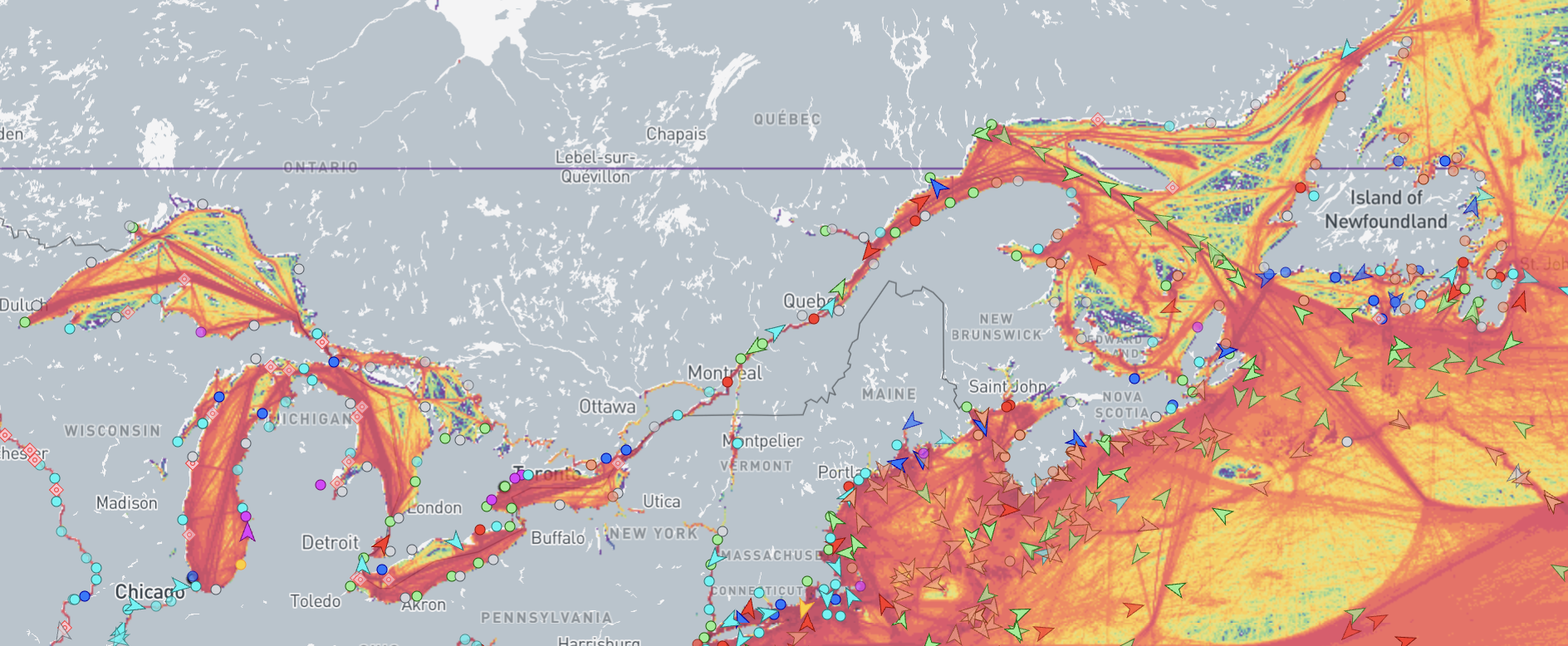
- The maritime space of the Great Lakes St. Lawrence region (GLSL) is a critical infrastructure
- Although the GLSL maritime corridor represents a small portion of the overall regional economy, it is an irreplaceable transport mode for many commodities
- Its growth potential is enormous
Problem
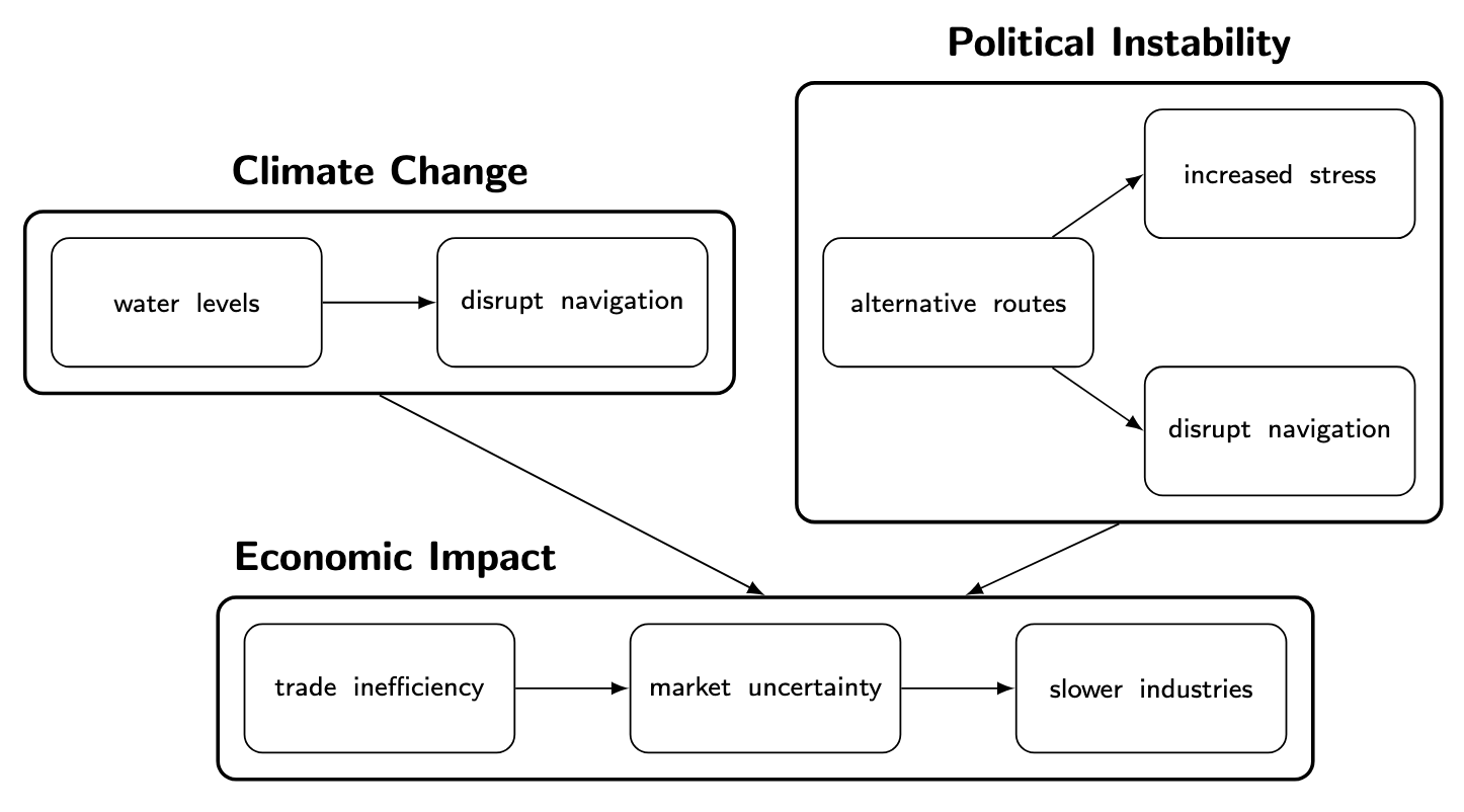
External Pressure

Internal Challenges
- Port network is decentralized as firms rent terminals to ports
- Port authorities manage demand and port calls locally in a decentralized manner
- → Lack of centralized logistics for port calls
The Graph and Network Theory Approach
What is a graph?
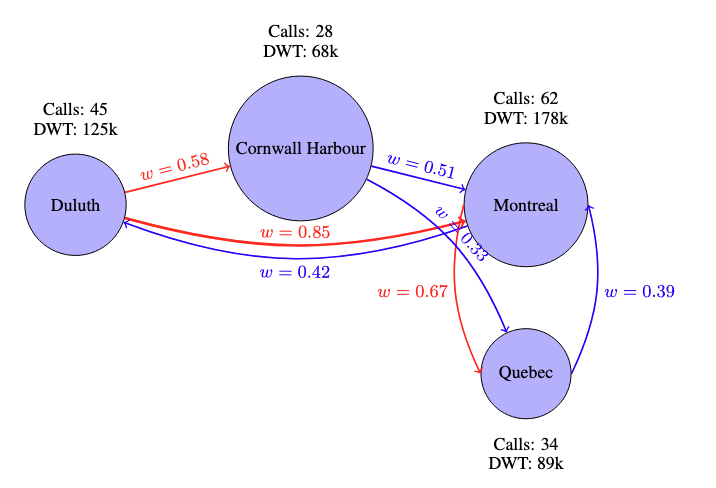
A graph is a mathematical structure consisting of:
- A set of nodes: Each node represents a port
- Node features: Deadweight distribution, port calls, ship type distribution, centrality, closeness, betweenness, PageRank, average dwell time, ship draft distribution, traveling time distribution, speed distribution
- Edges: A matrix representing the connections between nodes in terms of a certain metric. In our case, we use a weighted score of deadweight tonnage, trip count, and frequency to weight, or give a score of importance to each edge connecting nodes.
Example

Why is it best to think in terms of networks?
- Grasps the structure
- Understand interdependencies and optimize resource allocation
- Flexible, a graph is a model that can evolve
- Allows for node prediction, edge prediction, and counterfactual analysis
Expected Outputs
Node Prediction:
“How many port calls should we expect in Montreal for the next period?”
Edge Prediction:
“How many trips should we expect between Montreal and Quebec for the next period?”
Counterfactual Analysis:
What network representation allows us to do better than any other model like pure time series forecasting:
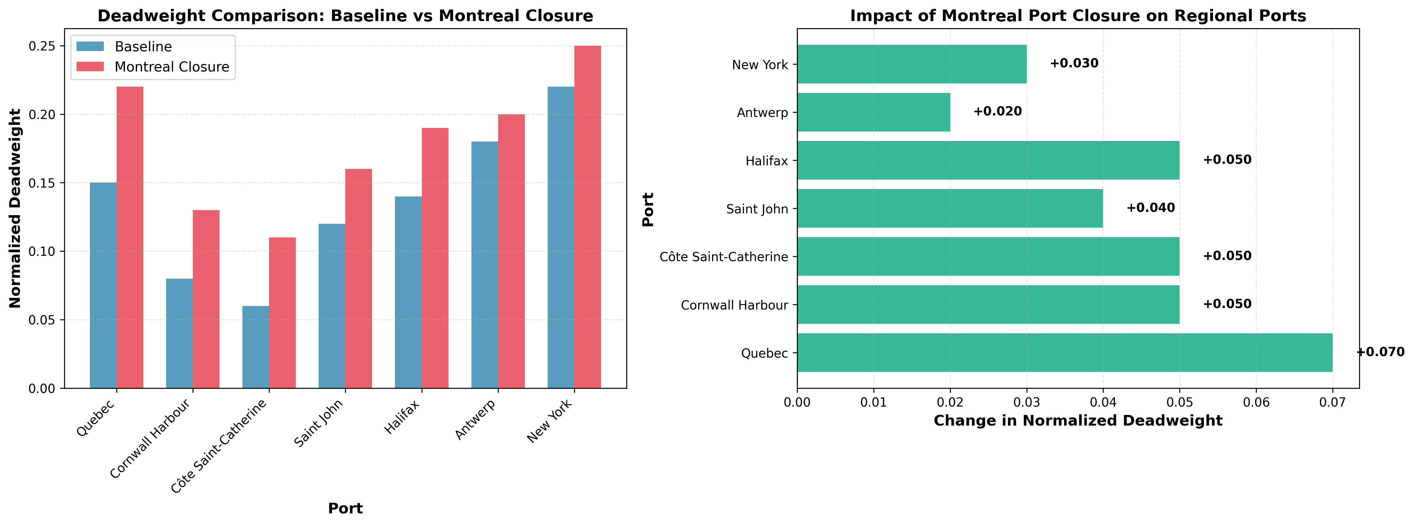
“What happens if port X closes? How could its load be redirected?”
“What happens if average draft decreases by 10% in port X in terms of deadweight capacity?”
Interactive 3D Network Visualization
Graphical Neural Networks (GNNs)
Training Set
Preliminary Results

Why Counterfactual Analysis is More Valuable Than Forecast?
- Time series can forecast future trends based on historical data
- Networks and graphs encode deeper information, the structure, and therefore are, in a sense, volume-agnostic (e.g., the volume traded in the GLSL maritime corridor can drastically change because of shocks, but the efficiency of a network representation is not impactedd by the shock)
Current Limitations and Perspectives
- Some structural variables at port level are missing (but to be included): equipment, terminal capacity, workforce, etc.
- Data on the commodities being transported are missing; this would help generate counterfactual scenarios based on shocks related to a specific industry
- We need more certainty about when a ship is empty or not
- This kind of model needs to be continuously updated with fresh data
- Graph sparcity needs to be further improved
- The learned graph structure will serve as a training environment for artificial agents (Reinforcement Learning)
- RL agents can learn in the actual learned graph structure from AIS data or on conterfactual graphs